In this chapter we dive into Big O Notation, a computer science concept that is vital for understanding the efficiency of algorithms. This is often a section buried deep in the back of a book, with a large scary disclaimer in front of it complete with complex math equations that seem meant to scare off the weak of heart. It is a deep and important topic, but I’m going to try to explain it in a way that’s not so intimidating. The idea is that you learn to see the general patterns represented by the most used equations, and how to apply them to your own analysis of algorithms.
I’m going to start this chapter with a confession: I hated math growing up. I once gleefully told my 12th-grade precalculus teacher that I would never need to know one single thing he taught me. Mr. Wittekind, on the off chance you’re reading this book right now, you were right and I was wrong.
In my biased opinion, and with a further apology to Mr. Wittekind, I think this has a lot to do with the way math is taught. Children are asked to memorize a bunch of formulas and concepts, without much of an idea of why they’re important or even what they are. If you ask most American high school students about algebra, they can likely tell you something vague about equations, quadratics, or slopes of lines. If you ask most American high school students “What is algebra?” I’m guessing they won’t know.
Unlike computer programming, it can be hard to make mathematical concepts immediately appreciable and understandable. I can teach you about a for loop, and then show you a cool example where you can make a computer say your name ten times. I can teach you y = mx + b and you might not understand why that’s important and useful to know for quite some time, if ever. It’s certainly hard to see immediately.
No wonder I was always drawn much more to computer programming than mathematics.
Now that I’ve got that out of the way, there is of course a strong link between mathematics and computer science. In many cases, the latest discoveries of one have been found thanks to ideas or methods derived from the other. This doesn’t mean you have to be a math whiz to be a great computer programmer, but a little bit of knowledge of math can certainly never hurt you.
Big O Notation is one of those little bits of math. You don’t need to solve long sets of problems or memorize lists of equations to understand and use Big O. There are some general principles you have to understand, and once you understand them you can add the Big O toolset to your arsenal.
What is Big O Notation?
Big O (from the German word “Ordnung”, or “order”) is a topic that can make developers tremble in their stylish sneakers. While the phrase “Big O” itself means something specific, which we’ll get to in a moment, what I mean by “Big O Notation” as used so far in this chapter is a set of equations that form curves on a graph. These curves usually represent time on the horizontal axis and the number of inputs to an operation — or set of operations — on the vertical axis. The “shapes” of these curves give developers a way to compare the efficiency of algorithms. Generally speaking, the flatter the curve, the more efficient the algorithm. What determines the slope of the curve is the number of operations that need to be performed to accomplish a given task.
For an example, imagine you and three friends go for dinner at a restaurant. The waitperson has only one “operation,” and that’s telling the kitchen staff what you want for dinner. Each of your orders can individually be considered an “input” to this operation.
Imagine the waitperson isn’t terribly efficient. He asks the friend across from you what they want for dinner, and then goes into the kitchen to tell the kitchen staff your friend’s order. He then comes back out and asks the person on your right what they would like for dinner, and runs back into the kitchen again to place the order. The waitperson continues around the table person by person, each time going into the kitchen to tell the kitchen staff what each person wants as soon as it’s ordered.
What does the curve look like? For each person at the table the waitperson has to go into the kitchen one time. Since there are four people at your table, the waitperson has to go into the kitchen four times. So this curve is a straight line, with the number of operations equal to the number of people at the table.
We’re going to get to the terminology later, but this operation is in “O(n)” time, where “n” is the number of people at the table. The shape of the curve is a straight line at a 45º angle. Kind of steep!
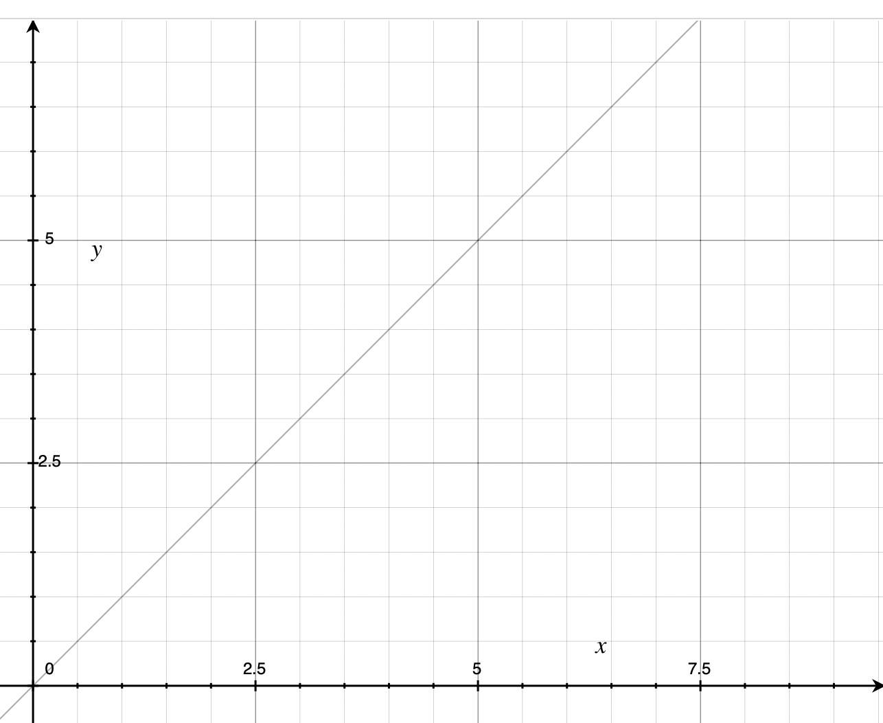
O(n)
Can we make this more efficient, and in so doing flatten the curve? Of course! If the waitperson asks everyone at the table what they want all at once, then goes into the kitchen with everyone’s order at the same time, the number of operations is reduced to one! This is a nice flat curve that describes one operation no matter how many people are sitting at the table.
Again, holding off on the terminology, this operation is in “O(1)” time, where “1” is the number of operations. This is also known as “constant time” because the number of inputs — people sitting at the table — doesn’t affect the number of operations required to place the order.
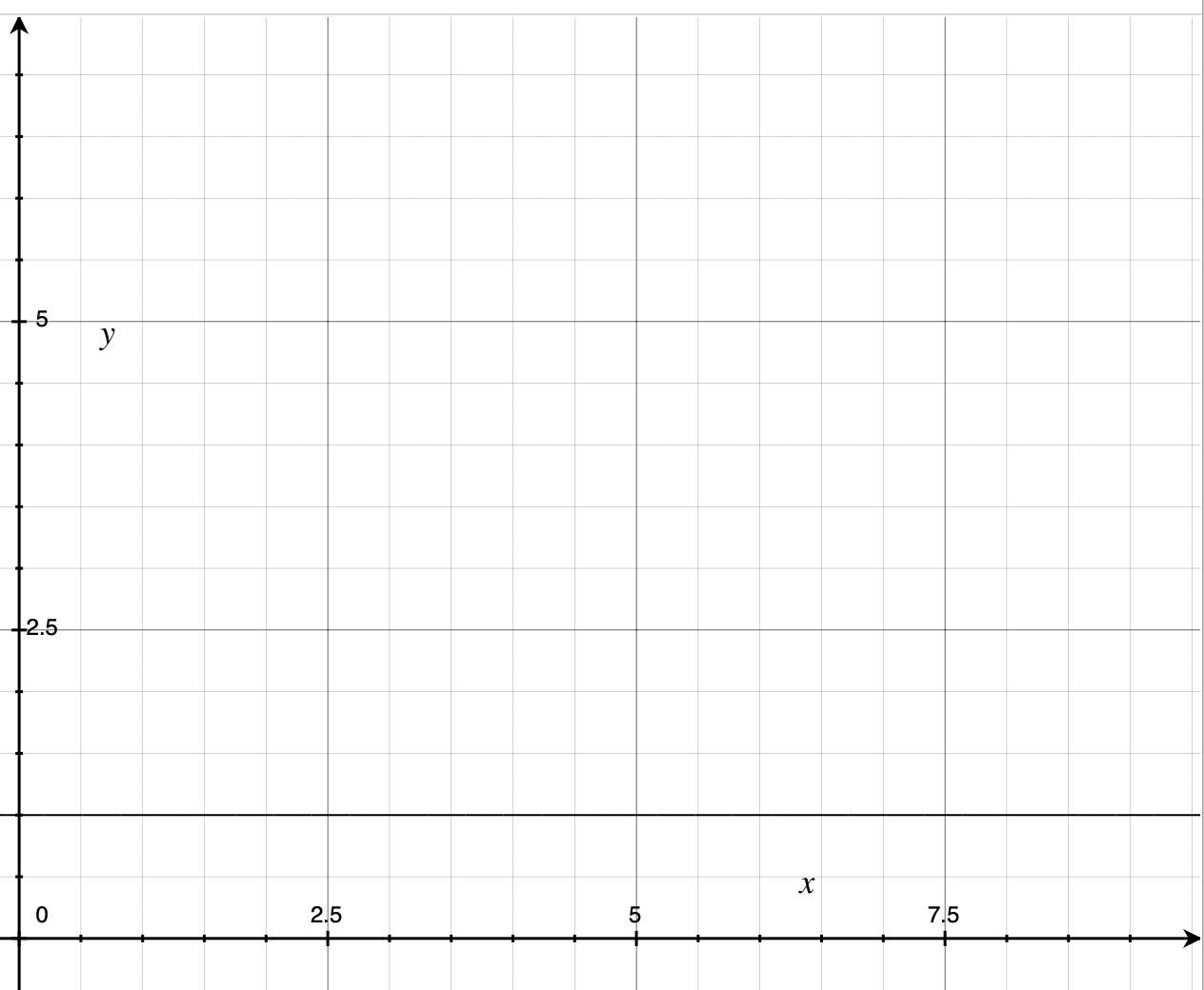
O(1)
This is exactly what Big O is for, analyzing the speed of algorithms. The most important idea behind Big O and related terms is that they measure speed in a general and relative, and not specific, way. What “general” means is that Big O is great for comparing algorithmic approaches or finding algorithmic optimizations.
What Big O is not used for is measuring exact run times — the “walk around the block” I mentioned earlier. The reason why is because computers can vary widely in terms of memory, running speed, available resources etc. So Big O is about seeing the overall trend of an algorithm, and not about getting a to-the-microsecond measurement of how long it takes to run. If you need to do that, programming languages and libraries contain execution and runtime timers that can tell you exactly how long something takes. Think of Big O as more of a benchmark. Big O is a bar that can be set to see if an algorithm can be improved.
Understanding Big O is a vital skill for getting through coding interviews, which is why this book is going to start with it. Rather than taking some crazy deep dive into every equation imaginable, I’m going to give you a few “Rules of Thumb” to keep in mind for a coding interview. These rules cover the most common Big O shapes you’ll come across, and according to an extremely non-scientific poll I never conducted, I would say that with these five shapes you can get through 80-90% of the Big O questions you’re likely to come across.
The Shapes of Big O
Let’s dive in. There are five Big O “shapes” you need to know. By “shapes” I mean slopes of a line on a graph, as I mentioned above but I think it’s easier just to consider them as shapes. If there’s one thing to memorize in this book, it’s these shapes — especially as they relate to one another. Yes, there are more. Yes, it’s more complicated than what I’m about to say. But if you can understand these five principles you’ve gained most of what you need to know to get through a coding interview.
I can’t promise you’re not going to be asked to explain how to derive Big O equations during your coding interview. But it’s unlikely. What you might be asked is to describe the efficiency of your algorithm in terms of Big O, and whether or not it can be improved.
In each of these graphs, the X or horizontal axis is the number of inputs. The Y or vertical axis is the number of operations that need to be performed to accomplish a given task. Usually, it’s not possible to decrease the number of inputs, so what makes an algorithm more or less efficient in terms of Big O is a reduction in the number of operations. As such, “flatter” graphs are generally preferred to “steeper” ones, as described below.
O(1)
O(1)
With O(1), no matter how many inputs you have, there’s only one operation that needs to happen. Generally speaking, it’s hard to beat this approach. Most algorithms don’t run with this kind of efficiency, but some do, and they’ll be discussed below. Notice that the shape of this graph is flat, and you can’t get more efficient than that.
O(n)
O(n)
Notice the shape of this graph. The number of inputs (x-axis) equals the number of operations (y-axis). An example of this is printing a list of names from a database. If there are 100 names, there will be 100 calls to print(). If there are a thousand names, there will be a thousand calls.
O(n) can be very efficient if there are only a few inputs. That’s a great place to start, but when you discuss Big O, you must always consider it at scale. If there are 100 inputs or one thousand, as mentioned above, it still might be more efficient than other approaches. But what if there are 500,000, or a million, or a trillion? The efficiencies of O(n) might diminish considerably compared to other approaches.
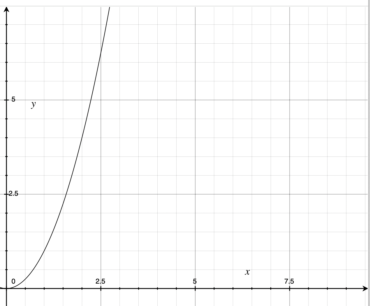
O(n2)
is the least efficient of all of the “shapes” discussed in this section. (also called “quadratic”) means that every operation must be done number of inputs multiplied by number of inputs times. If you have 100 inputs, it will take 1002 or 10,000 operations to complete the task. Notice that the shape of this graph takes off quickly and goes nearly vertical. The addition of even a small number of inputs will quickly cause the number of operations to skyrocket. An example of this happening is in nested for loops. Keep in mind that it gets worse than . Poorly built algorithms can take on or , etc., so try to avoid these approaches if you can. There are even worse metrics, including and . We’ll discuss these more later in this chapter and point out examples in the algorithms sections as they arise.
O(log n)
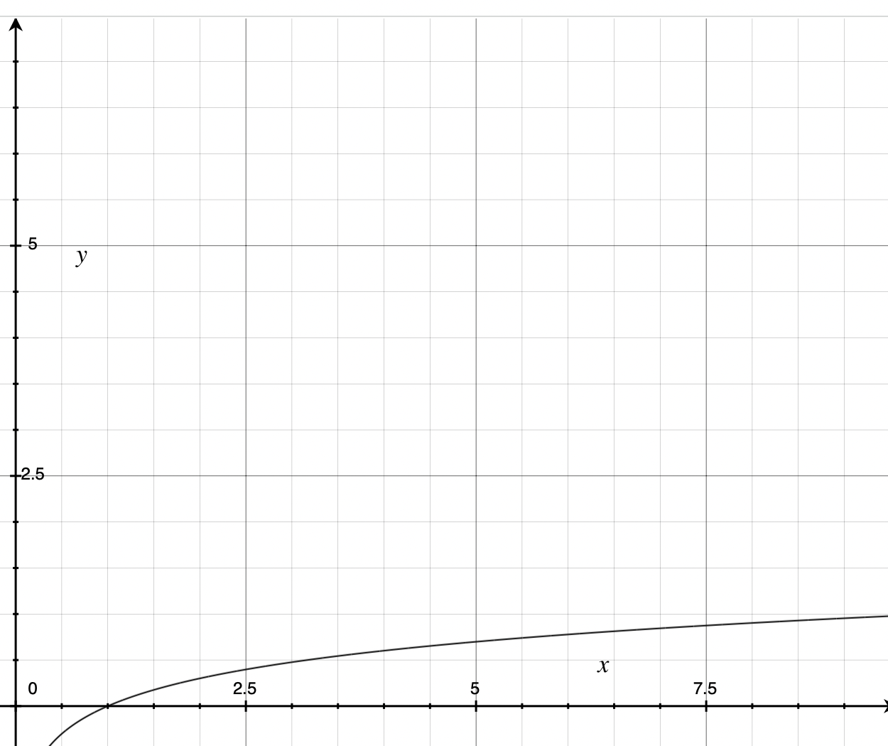
O(log n)
If you don’t remember logarithms from high school, a logarithm is the number something would have to be raised to in order to come up with a given number. To put that in a hopefully less confusing way, think about it like this: what would 2 have to be raised to in order to get 8? Since 23 is 8, the answer is 3 times, and so . There’s more to logarithms than this, of course, but right now we’re focusing on the shapes. Notice how slowly grows and flattens as it grows larger.
arises from algorithms that split the relevant number of inputs under consideration in half, repeatedly. You’ll soon see that this is the case with binary search and the height of binary trees. This is a highly desirable efficiency and one that should be sought wherever possible.
Closely related to is , which is less desirable than but certainly superior to . typically occurs when an algorithm performs a logarithmic operation for each of the inputs. Common examples include efficient sorting algorithms like Merge Sort and Quick Sort (average case). These algorithms divide the data (the part) but still need to process all elements (the part), resulting in operations total.
All of the shapes together
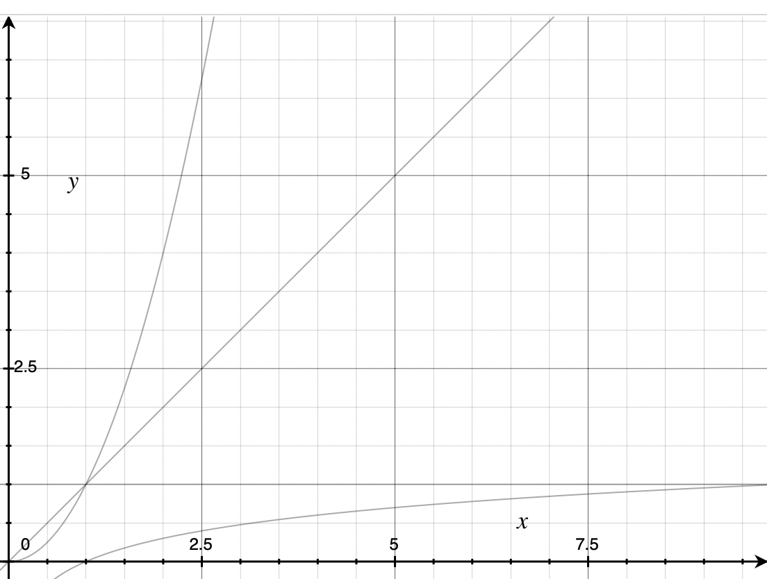
All Big O Shapes Together
Here are all of the shapes together. Take a moment and compare each shape to the others, and go back and re-read the description of any shape in isolation if you don’t understand what it means. These shapes are going to form the basis of the rest of the discussion of Big O, so really take a moment here if you need it. If someone asks you “Which is more efficient: or ?” you should see the two shapes in your head and immediately know the answer.
Nothing builds understanding like doing. If you want to cement the relationship between the equations in your mind, find a graphing calculator application or website and graph these shapes yourself. Zoom in and out on the graph and the points at which the lines cross, and come up with situations in which one operation would be preferable to another. Which shapes are better for smaller or larger numbers of inputs?
Discussion of Big-O
I started with the shapes so that you could keep them in mind as we discuss Big O in depth, so that it’s far less of an abstraction than what’s in computer science textbooks. Now that you’ve seen the shapes, it’s time to discuss in more detail what they mean.
Big O is a Limit
Big O is not about measuring the actual speed of an algorithm. For starters, that’s not an easy thing to do universally because different computers come in different memory and chipset configurations.
Big O is a type of “asymptotic analysis,” which is a mathematical way to describe limiting behavior. “Limiting behavior” means describing how an algorithm performs as the input size grows very large. For instance, when you buy a car you’re usually told what your expected gas mileage will be. This doesn’t mean your car will always (or ever) get this exact gas mileage. The number given is usually the absolute best the car can be expected to do, under a very specific set of conditions. But depending on any number of factors — passenger weight, tire pressure, weather, road conditions — your car won’t do as well as what the number promises. And no matter what, your car will not do better. So the gas mileage number describes a “limit.”
Technically, Big O describes an upper bound on an algorithm’s performance — the worst it can possibly do as input size grows. There are related notations: Big Omega (Ω) describes the best case, and Big Theta (Θ) describes the average case. However, in practice and in coding interviews, “Big O” is often used as a general term to discuss algorithmic complexity regardless of whether we’re talking about worst, best, or average case. This is not a book about formal asymptotic analysis, and there are a lot of them out there, so we’ll use Big O as a general term for algorithmic analysis.
To sum it up: if an algorithm runs in time, it will generally perform worse than an algorithm running in time, especially as the input size grows large. When comparing algorithms, the one with the “flatter” Big O curve will typically be more efficient for large inputs.
These descriptions should give you a sense that the idea behind Big O is to compare two approaches as generally “better” or “worse” in terms of expected performance.
Operations
In presenting the shapes to you I said that the X-axis represented the number of inputs, while the Y-axis represented the number of operations. It should be clear that the number of inputs is the number of pieces of data processed, but less clear is what is meant by the number of operations. More specifically, what exactly is an operation?
For the purposes of Big O, operations are the things that have to happen for the algorithm to execute. Because for the purposes of tech interviews Big O is about limits and not actual timing, think of an “operation” as a constant value. There could be three things happening, or four, or ten, but we’re more interested in how many times this group of things has to happen, than in the number of items in the group.
As an example, consider the multiplication table you may have learned in grade school:
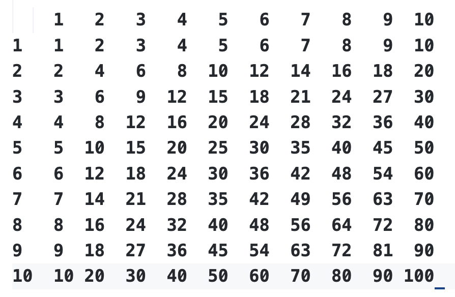
Multiplication Table
Here’s a general example of how this might be accomplished. Ignore the fact that there are no headers or proper spacing or optimizations and just focus on the fact the code contains a function definition, two for loops, and two print statements. There’s nothing complicated here: the code runs through two for loops and for each iteration through the loop prints out the number in the “i * j” position, much like the multiplication table itself does. The multiplication table in this form can be considered a “two-dimensional” piece of data.
def multiply(limit):
  for i in range(1, limit + 1):
    for j in range(1, limit + 1):
      print(f"{i * j}", end=" ")
    print("\n")
How many operations is this? You could consider that the function definition is one, the two for loops are two, and the two print() statements are two resulting in 5 operations. But as far as Big O is concerned, the answer is it doesn’t matter. For the purposes of Big O there are two for loops, which means that whatever you pass into limit, the number of operations in this code is , or times. The running time is .
What if you make the following modification to the code to add a header and a notification that the program has finished? Does this change the number of Big O operations involved?
def multiply(limit):
  print("Multiplication Table from 1 to ", limit)
  for i in range(1, limit + 1):
    for j in range(1, limit + 1):
      print(f"{i * j}", end=" ")
    print("\n")
  print("Finished!")
If all you’re adding is two lines of code, Big O remains at . Why? Because as I mentioned earlier, Big O is about the trend of the code running time, and not about the running time specifically.
So why is this important? It’s important because Big O allows us to talk about the optimization of code in terms of overall improvements to the running time of the algorithm. Again, because of the inherent differences between computers, the comparison between the running times of algorithms can be pretty meaningless. The multiply() function above is a very simple (I will not use the word “trivial” one single time in this book, other than right now) example that I picked to specifically illustrate , but as we go through this book we will see some algorithmic approaches that improve Big O in terms of either time or space complexity.
Pause and think: Can the multiplication example above be improved so it doesn’t use two for loops? Can it be improved so it doesn’t use for loops at all? Does this change the number of operations required to run this code?
Now that I’ve presented you with some introductory ideas regarding Big O, it’s a good time to consider some further specifics.
Constant Time
“Constant Time,” or Big O(1) means that the number of operations remains the same no matter how many inputs are passed to it. As such, this is a highly desired state of algorithmic optimization. It should come as no surprise to you, however, that it’s an incredibly hard state to obtain, and for some problems may simply not be possible.
Looking once again at printing the multiplication table above, no matter how you refactor the multiply() function, it’s going to have to run at . It has to in order to print the required numbers the required number of times. It cannot be optimized further.
But there will be examples in this book of starting with a “brute force” algorithm and optimizing that algorithm in order to flatten the curve. For instance, finding duplicates in an array can be improved from a brute force approach (comparing every element to every other element) to time by using a hash table to track elements you’ve already seen.
Logarithmic Time (log n, n log n)
Logarithmic time usually describes algorithms that split the data set in half with each iteration. For example, the Binary Search algorithm, discussed in Chapter 12, works by splitting the data set in half every time loop through the data is performed. The height of binary trees, discussed in Chapter 9, can also be derived logarithmically. Most (but not all) of the time we’re dealing with a base-2 logarithm, as is expected from a repeated reduction by half.
Logarithmic time can provide a significant improvement over polynomial times (see below) even if considerable algorithmic complexity is required as a result. There are algorithms that perform multiple complex steps but that might change complexity from a single step to three steps that are , , and in complexity, leading to the entire effort running in time. Such effort might drastically increase the complexity of the algorithm which now performs in three steps instead of one, but if you’re running thousands or millions of these operations — perhaps even in real-time — the short-term complexity is more than worth the long-term gain in speed. (We will not cover any such examples in this book, but look into the “Fast Fourier Transform” if you’re interested.)
Polynomial Time (, )
“Polynomial” time often occurs when the number of operations grows proportionally to the number of inputs raised to a power. The algorithm’s running time grows at a rate of , where is a constant, like or . While polynomial time is the most common algorithmic running time, it is not the most desirable, as it’s significantly slower than linear () or logarithmic () time. If your polynomial exponent is greater than 2 or 3, you’re in for a long wait. As shown in the multiplication example above, something that adds polynomial growth to the number of operations in an algorithm is a nested for loop. If you’re nesting for loops within for loops within for loops, you’ve missed something somewhere. That doesn’t mean it’s never the solution, but as a rule of thumb, if you find yourself taking a polynomial approach in an interview, that’s a pretty good sign that you’re missing an optimization somewhere.
Exponential Time () and Factorial Time ()
Beyond polynomial time, there are even more complex (and slower) algorithmic complexities that you should be aware of. While you’ll want to avoid these in production code whenever possible, it’s important to understand them for interviews because they often are the result of initial “brute force” algorithmic starting points before optimization.
Exponential Time ()
Exponential time complexity occurs when each additional input doubles the number of operations required. The classic example is the naive recursive Fibonacci implementation, where each function call spawns two more function calls:
def fibonacci(n):
    if n <= 1:
        return n
    return fibonacci(n-1) + fibonacci(n-2)
This creates a binary tree of function calls that grows exponentially. For fibonacci(5), you make 15 function calls. For fibonacci(10), you make 177 calls. For fibonacci(30), you make over 2 million calls!
Other examples include:
Finding all subsets of a set (the power set has subsets)
Brute force solutions to many optimization problems
Certain recursive algorithms without memoization
The growth is staggering: If you have an algorithm that takes 1 second for n=10, it will take about 17 minutes for n=20, and over 12 days for n=30. There’s not enough Red Bull in the world to get through that.
Factorial Time ()
Factorial time is even worse than exponential. This typically occurs when you need to consider all possible orderings or arrangements of n items. The classic example is generating all permutations of a string:
def permutations(string):
    if len(string) <= 1:
        return [string]
    result = []
    for i, char in enumerate(string):
        remaining = string[:i] + string[i+1:]
        for perm in permutations(remaining):
            result.append(char + perm)
    return result
For a string of length 3 (“abc”), there are 6 permutations. For length 10, there are 3,628,800 permutations. For length 13, over 6 billion!
Examples include:
The Traveling Salesman Problem (brute force: try every possible route)
Generating all permutations of a string, as just mentioned
Some brute force solutions to scheduling problems
In an interview you might be asked to solve a problem that has an brute force solution, but the interviewer expects you to recognize this and find a better approach. Being able to say “The brute force approach would be , so I need to think about optimization...” shows strong algorithmic thinking, even if you don’t immediately see how to accomplish it.
Be aware. If you find yourself writing an algorithm with exponential or factorial complexity, there’s almost always a better way, some of which we’ll cover later in this book.
Space
Big O notation in this book will refer to the complexity of the running time of the algorithm, as has been discussed throughout this entire chapter. It is possible, however, to also discuss Big O in terms of the space required to run the algorithm. Does the algorithm have to make a copy (or multiple copies) of the data to run, or can it use the existing data “in place” without the need for additional copies?
At the beginning of my career the internet was awfully slow, storage memory was a lot more expensive, and “plug and play” hardware had yet to come along, and so it was cheaper and faster to mail our spiffy presentations out to customers on 3.5" floppy disks than to ask them to sit through an hours long download. The capacity of a 3.5" floppy disk is just under 2MB. So everything we did had to fit within that memory space.
You might be glad those days are gone, but for programmers of embedded systems, microcontrollers or IoT devices memory can still be a precious commodity. So algorithms that unnecessarily duplicate data in order to process it may need to be optimized to handle space as well as time complexity.
Don’t be surprised if you go for an interview at a company that focuses on these types of products and you’re asked a question about improving space complexity. Even if you don’t plan to apply for these kinds of jobs, a 100MB web page is a bad practice that happens all too often because developers don’t understand space complexity. Computer memory is a lot cheaper than it once was, but that doesn’t mean it’s not precious!
Best, and Worst Case Complexities
For the last part of this chapter, I would like to focus on some different-than-best-case, um, cases. I briefly mentioned these above and will now expand a little bit on these different boundaries. The changes in boundaries can come from improvements to algorithms, or by using entirely different, better or worse algorithms, as you would expect. But they can also come from changes to the data. For instance, the Quicksort algorithm has an average case (Big O) of but a worst case (Big Ω) of . The only difference between the two cases is whether or not the data is already sorted. Because of the way the Quicksort algorithm works, it actually runs the slowest when the data is already sorted. This idea will be considered further when we examine Quicksort in Chapter 12.
Not all algorithms necessarily have a best and worst-case scenario. An algorithm that runs in constant time, for example, has a best case that is identical to its worst case.
Average Case (Big Theta (θ) Complexity)
This is also sometimes called the “exact case.” If you specifically measure every instance of every iteration of an algorithm and chart it, that could be considered an example of Big Theta. It would also result in a fairly crooked line that might represent a linear trend, or might show that the operating system speed is being adversely affected by having too many browser windows open. Because we’re looking to understand general trends and not exact algorithmic analysis, in this book Big θ will mean “average.”
Building Intuition: How is Big O used?
In coding interviews, Big O will usually be used to test one of two things: Do you understand the complexity of the algorithm you’re looking at, and/or can you reduce the complexity of the algorithm you’re looking at?
For example, you might be given a problem that requires you to sort an array. As a first option, you might choose to use the Quicksort algorithm which, as discussed above, has a worst-case running time of if the data is already sorted.
The questions regarding the complexity of Quicksort could come up in a number of ways: Do you know the average (Big Theta) time of this algorithm? Do you know the best-case (Big Omega) running time of this algorithm? Do you know of an algorithm that runs faster than Quicksort? What has to change for the Quicksort to become more or less effective? Do you know why Quicksort runs in Big O when the array is already sorted?
Example Questions
Here are some example questions you might be asked in a coding interview regarding Big O:
Refactoring for Big O
Since we haven’t gotten to the algorithms section yet, let’s consider another simple example of improving an algorithm in terms of Big O.
Imagine you have a drawer full of socks. All of the socks are identical, except half are white, and half are black. The room is dark and you need to find a pair of matching socks. What’s the most efficient way to do this?
You could reach into the drawer and pull out two socks, and then go out into the lighted hallway to see if they match. If they don’t, throw them in a pile on the floor and repeat the process until you find a matching pair.
If this is the way you choose to solve this task, there is no guarantee that you will ever find a matching pair!
Can you think of a way to improve this process? What if you compare the socks in your hand and keep the one in your left hand, discarding the one in your right hand if they don’t match? This is an improvement, but you could end up looking at half of the socks in the drawer before you find a match. That’s not a big deal if there are only 10 socks in the drawer, but what if you have, like, a million socks in the drawer? No good!
There is a guaranteed way to get a match on the first try no matter how many socks are in the drawer. If you grab three socks from the drawer right at the start, no matter what you are guaranteed to have a matching pair in your hands.
This is a Big O(1) solution to the problem, and you can’t get more efficient than that. In a coding interview, you might be asked similar questions about an algorithm and you should consider it in a similar way.
“This works if I have a small number of inputs, but can I be guaranteed a small number of inputs?”
“Do I have to grab only two socks at a time from the drawer?”
“Can I fix the light so I can just see the socks?”
As we get into the algorithms later in the book, I will be discussing the algorithms in terms of Big O, and will try to demonstrate how/why I came up with that particular Big O for that particular algorithm, and whether or not it can be improved.
Big O “Heuristic”
“Heuristic” is a fancy word for “trying a bunch of different things until you find one that works.” It can be challenging to optimize an algorithm for speed and efficiency, and until you gain some experience in writing algorithms, you are definitely going to want to make sure you’re able to be effective in terms of optimizing your code.
The first and most important thing you have to understand is what is the problem you’re trying to solve. If you don’t understand the problem you’re trying to solve the last thing in the world you should be doing is writing code. In the sample interview in the preface you’ll notice in the dialogue that the candidate is repeating the question back to the interviewer. This accomplishes two tasks: 1) It shows the interviewer that you’re a careful and active listener, and 2) It gives you a chance to slow things down so you can think about the problem for yourself.
Here are some basic steps to follow to optimize your code, whether you’re sitting in a coding interview or coding at work:
Put the problem into plain language. It does not matter how you do this. Write it down, say it out loud, draw a picture, whatever, but you need to say the problem in a way that allows you to comprehend what it is you’re trying to accomplish. In a work environment there might be time allocated to this, but in an interview you might have to just get this done on the side or in your head.
Start small. I started my career as a writer, and whenever I needed test data I would write very, very complicated test data sets. I thought it was genius because if the computer could handle a large, complicated data set, then surely the smaller, simpler sets would be no problem at all. Later I came to realize I was actually exactly wrong about this. I came to realize that I was making it harder for myself to just write good code, because I was always trying to solve a very specific, complicated, and unlikely problem. Instead of doing that, start with a small data set, and then build on that.
Do the smallest thing that could possibly work. This bullet is the same as the last one, except it applies less to the data and more to the code itself. The Agile software methodology suggests you start to “Do the smallest thing that could possibly work,” and that’s great advice. A lot of what developers spend their days doing is breaking large, intractable problems down into smaller, more manageable problems and then solving those. Take this same approach in a coding interview. Don’t try to knock the whole problem out of the park in one swing. You’ll likely end up with a large tangle of code that doesn’t work and is hard to understand and either you or the person hired to replace you will have to spend a lot of time either debugging it or throwing it out and rewriting it.
Start with a brute force solution. Start writing some code that solves the problem in the most straightforward way you can come up with. Do not try to start with optimization. Unless you see the optimization immediately, you’re much better off getting something down that works and then going back through the optimization process with the interviewer. Again, the trick is to start small. Get the code working first, and then the optimizations will suggest themselves.
Look for improvements. An important part of being successful in a coding interview is “pattern recognition,” a theme that will be returned to throughout this book. Nested for loops? That can probably be improved. Repeatedly calculating the same information? You can definitely get the time down on that. Once you’ve got the basic code down it’s a lot easier to see where the things are that can be done better. If you’re not sure, you can always ask the interviewer if there’s a way to improve the code. Plenty of examples of moving from brute force to a more optimized solution will be given in the algorithms section of this book.
Remember the “shapes” of the Big O Curves. Once I was in a large team meeting where a very smart developer pointed out that a solution a team member had come up with was “quadratic.” No one knew what he meant, and no one raised their hand. As mentioned just above, “quadratic” means the multiplication table, nested for loops, ! Often — not always but often — quadratic solutions can be improved. Once you recognize that this is the case, even if you can’t figure out how to improve the code, you can at least identify the problem, and signal to the interviewer that you’re aware of the issue.
Example Questions
Think of a simple (or complex) everyday situation you might encounter, and think about how it might be improved. For instance, I used to work in a print shop with an offset press, and whenever we had to print a two-sided document, I would stand at the output tray turning every sheet of paper over one at a time as it came out. A senior employee pointed out to me that if I just waited until the end and turned the whole stack over at the same time, I could improve my efficiency. What Big O shape is my approach? What Big O shape is the improved approach?
Find an algorithm you’ve written in the past and analyze it in terms of Big O. Can you find an optimization?
In an interview, you might be asked to analyze an algorithm in terms of Big O, be it your own or one that’s given to you, and asked for ways to improve it. You might also be asked to compare two algorithms in terms of Big O and asked which is more efficient, and why.
Food for Thought
Big O is the kind of topic people either love or hate. Some coders like to get down in the weeds on what the subject has to offer, and some avoid it like poison oak. If you really want to understand Big O, there are a lot of great resources out there, starting with the Wikipedia page on Big O Notation. If math is your thing, the course that got me to really see the Big O “big picture” is MIT’s “Mathematics for Computer Science” course, which is available for free online in the MIT OpenCourseWare series on YouTube. That’s not a beginner course and some prior knowledge of math — specifically algebra and basic calculus — is assumed, but if your goal is to “go there” on Big O, this is just where to go.